By: Philip B. Erlanger, CMT
"Trading Seasonality" - Introduction
Wall Street research is fraught with techniques to aid traders and investors in the pursuit of the Holy Grail - a set of indicators that will guarantee a steady return. Some of these techniques truly add value, some don't. The problem is that the stock market is a non-linear environment; the factors that influence price action are complex. No single combination of factors exists that perfectly repeats over time. Like life, the factors that influence stocks have infinite possibilities. It is up to each trader to determine which factor to value in the decision making process (a fact that in and of itself adds to the non-linearity of price action.)
Most of Wall Street research indicators are linear attempts to solve a non-linear problem. Some try to turn one factor into a science. Others look at so many factors that any value is lost by the effect of diminishing degrees of freedom. The trader must therefore decide which factors are of most value. We choose factors that are primarily of a technical nature. Technical analysis is research derived from the action of the marketplace itself. The types of technical indicators we use include those derived from price action, volume changes and sentiment. We value those factors that are independent of other factors, have a reasonable degree of correlation to price action, and that successfully repeat over time. Perhaps the most misunderstood and least used of these factors is seasonality. Over the years the more we have used seasonality the more we have come to value it as a primary factor in our decision making. Here's why.
What Is Seasonality
In general, seasonality is some repeatable tendency of a financial instrument to move in relation to a particular influencing factor. That factor could be the time of year, the year of a decade, changes in interest rates, inflation, energy prices, etc. We focus on stock price action and seasonal cycles derived from the time of the calendar year.
Seasonal cycles do not cause prices to move a certain way. They simply reflect a measure of tendency. Ongoing price action is influenced by many factors, only some of which occur on a regular, repeated basis. Those factors that regularly cause a stock price to move a certain way at a particular time of the year may or may not be known, but their seasonal influence will show up in the seasonal indicators and can be qualified by several techniques to measure the breadth and consistency of a stock's seasonal pattern.
When entering into a trade, there are two basic types of indicators: setups and triggers. Seasonality is a setup indicator. Setup indicators are designed as filters that steer the trader to moments when making a trade will result in greater success than others. Examples of setup indicators other than seasonality include sentiment (a contrary setup indicator,) industry group relative performance, fundamental information (e.g. earnings momentum) and price, volume, or other "divergence" oscillators (e.g. Relative Strength Index or "RSI," Moving Average Convergence/Divergence or "MACD," or Erlanger Volume Swing.) Oscillators are used as setups most often when they begin to diverge from price action. For instance, if price is rising to a new reaction high unconfirmed by the RSI oscillator, a setup for a potential short sale exists. Triggers are designed to tell the trader the exact moment to execute a trade by measuring when price begins to move in the direction indicated by setup indicators. Examples of triggers include moving average crossovers, price moving through a DMA (displaced moving average) channel, or a change in status of a trend direction indicator. Some indicators, like the MACD are used as both setup and triggers (setup when the MACD diverges with price, trigger when the MACD crosses its signal line.)
The trading process typically begins with the prelude of one or more signals from setup criteria, and then the trade is made when the market moves sufficiently in the anticipated direction to set off the trigger indicator. After the entry trade, "monitoring" indicators are used to exit the trade. These "monitoring" indicators can in some instances be the same indicators used for set-up or trigger events, or they can be a completely different set of indicators or indicator criteria. For instance, one can trigger a long position if price moves above the 10-day moving average, but "monitor" the position and sell only if price falls below the 21-day average. The indicators and criteria are up to the individual trader's style and preference.
Stock price changes are what the trader tries to exploit. At the end of the day the successful trader either buys at a lower price than sold, or sells short at a higher price than covered (buying to close out a short position.) Setup and trigger indicators therefore generate information for either direction of an opening trade (long or short.) Seasonality uncovers those moments when the market or stock tends to rise (a set up for long trades) or fall (a set up for short trades.) The beauty and marvel of seasonality is that it is known so far in advance, and yet still has value as a timing mechanism. We know of no other stock market factor that has this feature. Let's step through the process of developing seasonal statistics for stocks, and examine how effective they can be for trading purposes.
The Yearly Seasonal Cycle
There are many time periods one could use to create seasonal cycles. In fact, all cycle analysis is in reality an effort to measure seasonality. We could look at 10-year, 20-year, monthly, weekly, daily, even hourly periods in an effort to uncover repeating patterns. For the purposes of this exercise, we will focus on uncovering seasonal patterns associated with daily closing price action over the calendar year.
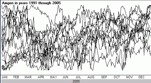
Figure 1 Amgen (AMGN) from 1991 through 2005 spliced up into yearly lines
Figure 1 shows the first step in preparing a seasonal cycle. We have chopped up the 15-year history of Amgen Corp (AMGN) and plotted each year starting January 1 through to the end of December. At first brush it looks like spaghetti, or for the more imaginative it might serve as some sort of Rorschach inkblot test. However, by compositing these years into one linear curve, a seasonal cycle is born.
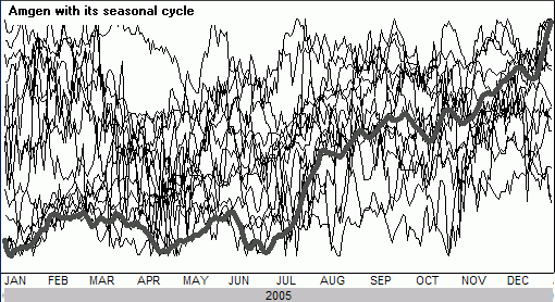
Figure 2 Amgen with its seasonal cycle
The number of years used to create a seasonal cycle is subjective. Enough years are needed to establish a statistically valuable pattern, but too many years could add old and possibly outdated information. We look back 15 years as a default, and then do a moderate process of optimization to find the best, most recent period of data to use. Optimization can be injurious to good results when testing for signals in stock data indicators. This is especially true if criteria or parameters are set as a result of excessive optimization techniques. The danger is one of curve fitting, where the indicators are parameterized to work well with a specific body of data, but are ineffective outside in the real trading world. However, here we are doing something a bit different. In any sample of data there is going to be a composite cycle. The key is to find a composite cycle that is a repeating pattern. We do this by taking a large enough sample (up to 15 years.) We then split this sample in half and create two additional composite cycles - one from the first half and one from the second half. If these two "mini" cycles are somewhat correlated, than we have greater confidence that the original cycle represents true seasonality. Optimization comes in by adjusting the original sample size to maximize the correlation of that sample's "mini" cycle halves. Let's look at an example.
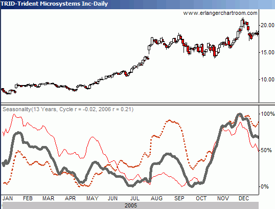
Figure 3 Trident Microsystems (TRID) with its "mini" cycles - 13 year sample
In Figure 3, does the seasonal pattern reflect tendencies throughout the 13-year history of Trident Microsystems (TRID), or is it a random cycle? To answer this question, we create the two "mini" seasonal composites, one from the first half of TRID's 13-year history (1993 to 1998 - see thin line in Figure 3), and one from the second half of TRID's 13-year history (1999 to 2005 - see dotted line in Figure 3.) We only use complete years in constructing seasonal cycles. If the sample size is an odd number of years, we add the median year to the latest "mini" cycle composition. The thick line is the seasonal cycle based on all 13 years of TRID price history. All these cycles bear similarities, especially at certain times of the year (the high points in late January and early December and the low point in mid-April, for instance.)
We use a correlation statistic called Pearson's R. Pearson's R is a statistical expression of linear relationship between two variables. It ranges from +1 to -1, with a reading of +1 being a perfect match between two variables. A reading of -1 indicates a perfectly inverse relationship between two variables, while a reading of 0 implies no relationship or correlation at all between the two variables. In Figure 3 in the caption is a "Cycle r" statistic. This is the Pearson's R of two variables, the seasonal cycle for TRID based on years 1993 through 1998 (thin line) and the seasonal cycle for TRID based on years 1999 through 2005 (dotted line.) In this case the Cycle r equals -0.02, implying no correlation. Our conclusion from this is that the yearly cycle derived from the entire 13 year history has too much noise in it to be very effective. "Noise" in the data reflects price action that is random and obscures the clarity of the seasonal pattern we are looking for. However, many of the turning points of the 13-year cycle do seem to match well with the price action in 2005. We have observed that cycles with a "Cycle r" statistic around zero have some worth when looking for turning points. We eschew cycles whose "Cycle r" statistic correlations are negative. These indicate a composite where conflicting patterns exist: there is too much noise in the data to expect future price action to follow the cycle.
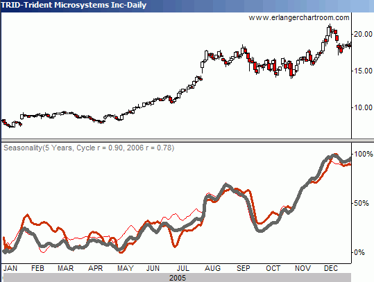
Figure 4 Microsystems (TRID) with its "mini" cycles - 5 year sample
Faced with a "Cycle r" statistic of -0.02 for our 13-year sample cycle for TRID, we can decide to look at shorter sample periods to find a higher "Cycle r" statistic, and perhaps a more significant seasonal pattern. The sample with the highest "Cycle r" statistic turns out to be of 5 years duration. Because this is a shorter sample period, the persistence of this seasonal pattern is considered to be statistically "local" - that is, less representative of longer-term cycles. Nevertheless, the trade off is a much higher "Cycle r" statistic of 0.90 (see Figure 4.) In this 5-year pattern, the "mini" cycles are highly correlated. Interestingly, the key turning points found in the 13-year cycle (the high points in late January and early December and the low point in mid-April) clearly remain in the 5-year cycle.
Seasonality Zones
Since we are putting our computer to work, let's have it highlight those 14-day (or longer) periods in the seasonal cycle that are strongest "zones" and also highlight those 14-day (or longer) periods in the seasonal cycle that are the weakest "zones."
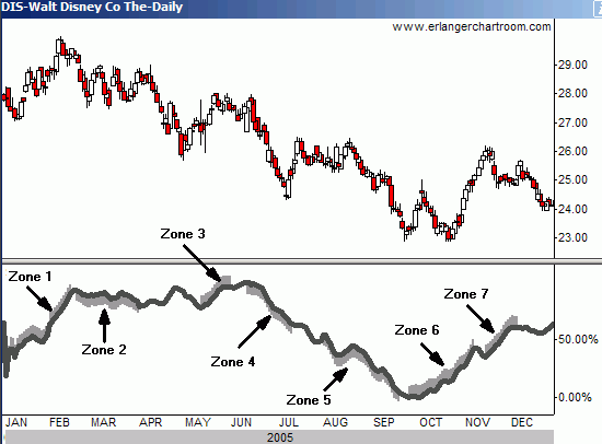
Figure 5 Disney (DIS) seasonal cycle with seasonality zones
These zones are plotted in Figure 5 for Disney (DIS). In this chart, the seasonal cycle uses a 14-year sample from 1991 to 2004. This particular cycle was created on January 1, 2005 and was not changed in any way as 2005 actually transpired. In other words, the seasonal cycle you see below Disney's 2005 price action was created using data prior to 2005, and it was up to the price of Disney to follow it or not to follow it. The computer program has added shading to highlight the seasonality "zones." Shadings on top of the seasonal cycle represent the strongest seasonal periods of 14-days or longer. Shadings below the seasonal cycle represent the weakest seasonal periods of 14-days or longer. Note how the price of Disney moved during 2005 relative to these "zones."
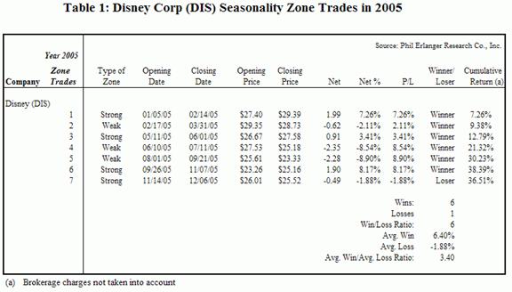
Table 1 contains the data for all the seasonality zones for Disney in 2005. There were 7 zones in 2005, four strong zones and 3 weak zones. Remember that these zones were identified with data ending in 2004. The price action of Disney in 2005 remarkably followed the paths of these zones in 6 out of the 7 instances. Not including commissions, the cumulative return in Disney's stock price during these zones was 36.51%. For 2005 as a whole, Disney's stock price fell 3.83 points, or -13.78%. For Disney in 2005, trading the seasonality zones outperformed a buy and hold strategy by 50.29% (36.51% - (-13.78%).)
Seasonality Heat
We have discussed seasonal cycles, but the fact of the matter is that they are simple guidelines to past behavior during specific periods. Seasonal cycles are composites of past price action, and as such they "hide" measures of seasonal consistency throughout the price action's history. We can adjust the historical look back period to optimize for Cycle "r" as discussed above, but this optimization process tells us more about the validity of the seasonal pattern than it does about the consistency of the seasonal pattern. Our "seasonal heat" process is designed to address the need to measure seasonal consistency.
At the beginning of each New Year the seasonal cycle is updated with new seasonality zones, incorporating information from the just completed prior year's data. While these seasonality zones do not appear precisely at the same time intervals each year, they typically do not deviate greatly from past years. This is at least the case for stocks that have strong seasonal tendencies. The key is to identify those moments in time when seasonality zones of prior years most often occur. For any given day of the year, the more frequently seasonality zones have occurred in past years, the greater the "seasonal heat" is (in our charts seasonal heat is greatest when the background coloring is brightest.) Seasonal heat can be either positive or negative. Positive seasonal heat is a greater number (brighter background color above the 50% line in the charts.) Negative seasonal heat is a greater negative number (brighter background color below the 50% line in the charts.)
Figure 6 Disney with Seasonal Heat Map
Figure 6 shows the Disney chart with the seasonal heat map added. Positive seasonal heat is shown above the 50% line; negative seasonal heat is shown below the 50% line. Looking at the heat map above the 50% line, the brightest sections correspond to those periods most frequented by strong seasonal zones in prior years. This illustrates the consistency of seasonality. The more a seasonal pattern repeats, the more likely it is to occur in the future. This is true for strong and weak seasonal patterns. Moreover, those periods in a seasonal map during which the positive seasonal heat is absent (darkest) are potentially riskier moments for Disney than other times of the year. This was certainly true in 2005, as Figure 6 demonstrates.
Let's take the concept of seasonal heat a bit further, and examine all the Dow Jones Industrial Average 30 component issues during 2005. We will confine our strategy to buying these issues only during the strongest seasonal zones that have the most positive seasonal heat. In a case where there are two strong seasonal zones with similar extremes in seasonal heat, we will count both as trades. The same goes for short sales. We will confine our short selling strategy to shorting issues only during weak seasonal zones that have the most negative seasonal heat. In the case where there are two weak seasonal zones with similar peaks in seasonal heat, we will count both as trades. Table 2 shows the results.
Table 2 Dow Jones 30 Issues Seasonality Zone Trades in 2005
The results for 2005 are striking. Out of 69 trades, 55 were profitable resulting in a win/loss ratio of 4:1, an average win to average loss ratio of 1.97:1, with average wins equal to 7.05% and average loss equal to -3.57%. The average trade yielded a 4.90% gain. The maximum gain was 22.50%, and the maximum loss was -7.94%. For the year of 2005 as a whole, the Dow Jones Industrial Average itself lost -0.61%.
Seasonality and Other Instruments
Seasonality analysis need not be confined only to stocks. Any instrument that has enough price history can be the subject of seasonal analysis. For instance, the price action of one stock relative to another stock (called pairs trading) can exhibit seasonal patterns. Let's examine the Pepsi (PEP) versus Coca-Cola (KO) pair.
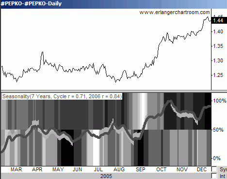
Figure 7 Pepsi/Coca-Cola pair with seasonal patterns
The seasonal cycle for the Pepsi/ Coca-Cola pair in Figure 7 is relative flat until September, when it rises sharply with maximum positive seasonal heat. The pair itself rises when the stock price of Pepsi outperforms the stock price of Coca-Cola. Since the seasonal pattern favors a rise in the paired trade starting in September, traders would expect a "long Pepsi/short Coca-Cola" trade to be setup at this time. Indeed, in 2005 the Pepsi/ Coca-Cola pair did rise from 1.24 on September 7, 2005 to 1.39 on October 19, 2005, when the seasonal cycle flattened out just prior to a weak seasonal zone.
Seasonal analysis can be performed on other indices. Industry group, sector and market indices are prime examples. Many professional money managers believe that the influence of groups, sectors and the stock market itself play a large role in the path taken by individual stocks. We agree, and constantly apply our seasonal microscope to such indices.
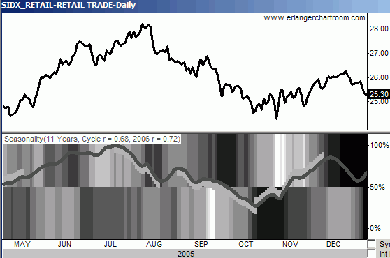
Figure 8 Retail sector seasonal patterns
Figure 8 shows the seasonal pattern of the retail sector. The retail sector is a composite of many industry groups related to retail sales, including building material chains, catalog and specialty chains, clothing/shoe/accessory chains , computer/video chains, department stores, discount chains, drug store chains, food chains and other miscellaneous retail chains. These diverse retail industries are reflected in the one retail sector index. As Figure 8 shows, the 11-year seasonal cycle of the retail sector has a high Cycle r statistic of 0.68, indicating the presence of a valid seasonal pattern throughout the past 11 years. There are also moments of strong seasonal heat, indicating consistency of seasonal zones appearing at the same time in prior years. This information is invaluable to professional portfolio managers who often make sector and industry group money management decisions.
In Figure 8, we see a seasonal pattern of weakness for the retail sector in September, followed by strength in October and November. As it turns out, this is similar to the seasonal pattern of the market as a whole, but the task now becomes one of finding retail industry groups and particular stocks that strongly follow the seasonal pattern of the retail sector. In general, most of the retail groups follow this pattern, but the clothing/shoe/accessory chains appear to most suitably mirror the September through November retail sector seasonal setup.
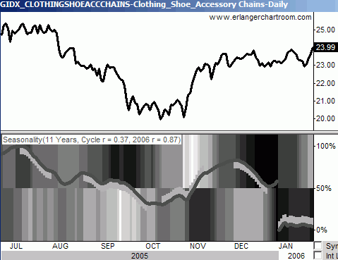
Figure 9 Clothing/shoe/accessory chains with seasonal patterns
In a similar fashion to the seasonal data derived from the retail sector index, Figure 9 shows a weak seasonal curve in September for clothing/shoe/accessory chains, with a large degree of negative seasonal heat. This turns around in the October and November period, with November showing a large degree of positive seasonal heat for clothing/shoe/accessory chains. As it turned out, the 2005 price action of the clothing/shoe/accessory chains followed this pattern closely. The task now becomes finding stocks that show comparable seasonal tendencies.
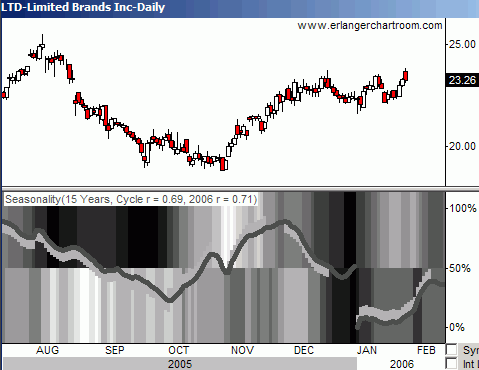
Figure 10 Limited Brands (LTD) with seasonal patterns
Figure 10 shows the seasonal pattern for Limited Brands (LTD), a major retail stock from the clothing/shoe/accessory chains industry group. This is a good candidate because its seasonal curve follows the path taken by its group and sector (and of course the market as a whole,) and also because its seasonal heat patterns of the current seasonal zones show great consistency with seasonal zones of the past. Moreover, the Cycle r statistic over the past 15 years is a highly correlated 0.69, which means the seasonal pattern is valid over the 15-year look back period. In truth, there are a number of individual retail issues that qualify as portfolio candidates using such seasonal criteria. It is the job of the portfolio manager to sift through the candidates and select those that meet seasonal and other criteria as befits the manager's style.
Deploying Seasonality as Part of an Overall Strategy
Seasonality is a powerful technique that portfolio managers should employ. However, no one factor should dictate strategy. A sound strategy uses setup indicators and trigger indicators, and follows up with a reliable monitoring mechanism to aid in exiting trades. Seasonality is primarily a setup mechanism. Other setup mechanisms include (but certainly are not confined to) measures of sentiment. For instance, the observation of short sellers can uncover moments in time when either the bulls or the bears are particularly at risk from contrary move - hence the setup. Let's return to our example of Amgen to illustrate the point.
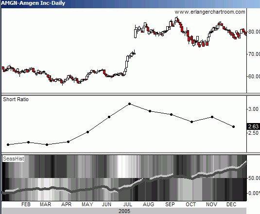
Figure 11 Amgen (AMGN) with short ratio and seasonal patterns
Figure 11 highlights two factors that show Amgen may be set up for a 3 rd Quarter buying opportunity. The seasonal curve turns up on June 24, initiating a positive seasonal zone. Seasonal heat is also very positive. In addition, the short interest ratio has swelled significantly during 2005 heading into this positive seasonal period. Clearly these short sellers are either unaware of or are ignoring, the seasonal tendencies of Amgen. In a matter of days from the strong seasonal zone that started on June 24, 2005, Amgen took off, activating any short-term trigger indicators one might employ. The ensuing "short squeeze" included a huge gap to the upside and peaked 87 days later on September 19, 2005, just days after the completion of the second strong seasonal zone. This action handed the bulls a 40.53% gain.
Of course it is wonderful when the market follows those factors we employ. The market, however, is not so easily tamed. Its non-linear nature assures us of many moments when unforeseen factors rise up and bite us in tender places. Ironically, one of the most valuable observations that can be made of set up indicators is to recognize when they fail to work. Such moments indicate an unforeseen factor is in play - a factor that is more meaningful to the marketplace. When indicators fail, it means another game's afoot; this is a clue to the portfolio manager that adjustments are needed. At the very least a failed indicator should taint the manager's bias (either long or short.)
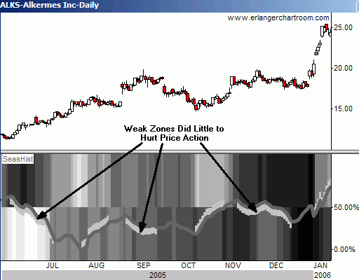
Figure 12 Alkermes (ALKS) with its seasonal patterns
Consider the seasonal pattern of Alkermes in Figure 12. The June weak seasonal zone is accompanied with blazingly negative heat. Nevertheless, price action rallied during this period. (Incidentally, trigger indicators would have kept traders from shorting here, because price action was so positive.) Clearly something else is biasing the action in Alkermes price - a clue for portfolio managers to be biased to the long side. As it turned out, Alkermes was in the midst of a long-term uptrend peppered with only the briefest and most moderate of pullbacks. All three weak seasonal zones in Figure 12 did little to hurt price action. These failures were clues to expect more than average performances of the strong seasonal zones.
Conclusion
Seasonality is a phenomenon that is measurable, but it is not a causal factor. Seasonal cycles do not cause markets to move. They are rather a function of other factors, known or unknown, which over and over again influence the direction of stock prices. We believe that if traders limit their trading to those periods where seasonal tendencies are consistent, the chances of post "trigger" success are better than otherwise.
As is true with most of the areas of Wall Street analysis, more research needs to be done in the areas of technical analysis in general and seasonality specifically. We hope this text encourages many to pursue their understanding and experience with seasonal trading.